44 how to change data labels in excel 2013
VBA to change data label in a chart - Compatibility btw Excel 2013 and ... It seems that Excel 2010 and 2013 work differently regarding to number format code in Macros. Due my limited access to Excel 2010, the solution was to duplicate the charts, change the labels as necessary and then switch the macro to show only the charts with the millions/thousands labels. Custom Data Labels with Colors and Symbols in Excel Charts - [How To] Step 4: Select the data in column C and hit Ctrl+1 to invoke format cell dialogue box. From left click custom and have your cursor in the type field and follow these steps: Press and Hold ALT key on the keyboard and on the Numpad hit 3 and 0 keys. Let go the ALT key and you will see that upward arrow is inserted.
Excel Barcode Generator Add-in: Create Barcodes in Excel 2019/2016/2013 ... Create 30+ barcodes into Microsoft Office Excel Spreadsheet with this Barcode Generator for Excel Add-in. No Barcode Font, Excel Macro, VBA, ActiveX control to install. Completely integrate into Microsoft Office Excel 2019, 2016, 2013, 2010 and 2007; Easy to convert text to barcode image, without any VBA, barcode font, Excel macro, formula required

How to change data labels in excel 2013
How to change chart axis labels' font color and size in Excel? We can easily change all labels' font color and font size in X axis or Y axis in a chart. Just click to select the axis you will change all labels' font color and size in the chart, and then type a font size into the Font Size box, click the Font color button and specify a font color from the drop down list in the Font group on the Home tab. See below screen shot: How to Change Excel Chart Data Labels to Custom Values? You can change data labels and point them to different cells using this little trick. First add data labels to the chart (Layout Ribbon > Data Labels) Define the new data label values in a bunch of cells, like this: Now, click on any data label. This will select "all" data labels. Now click once again. How to Print Labels from Excel - Lifewire Select Mailings > Write & Insert Fields > Update Labels . Once you have the Excel spreadsheet and the Word document set up, you can merge the information and print your labels. Click Finish & Merge in the Finish group on the Mailings tab. Click Edit Individual Documents to preview how your printed labels will appear. Select All > OK .
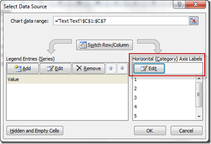
How to change data labels in excel 2013. Changing Axis Labels in PowerPoint 2013 for Windows - Indezine Now, let us learn how to change category axis labels. First select your chart. Then, click the Edit Data button as shown highlighted in red within Figure 7 ,below, within the Charts Tools Design tab of the Ribbon. This opens an instance of Excel with your chart data. Notice the category names shown highlighted in blue. Figure 7: Edit Data button Move data labels - support.microsoft.com Click any data label once to select all of them, or double-click a specific data label you want to move. Right-click the selection > Chart Elements > Data Labels arrow, and select the placement option you want. Different options are available for different chart types. excel - Change format of all data labels of a single series at once ... Workaround 1: Fill up all empty cells referred to. Change the format of labels. Remove added contents. Workaround 2: Change to a dummy range for the data labels, which has no empty cells. Change the format of labels. Switch back to your intended range. How to rotate axis labels in chart in Excel? - ExtendOffice If you are using Microsoft Excel 2013, you can rotate the axis labels with following steps: 1. Go to the chart and right click its axis labels you will rotate, and select the Format Axis from the context menu. 2.
Convert Address Labels from Word 2013 to Excel 2013 The data originally came from a PDF that I converted to Word 2013. The format for each name is as follows: Full Name. Address 1. Address 2. City, State, Zip. On about half the records, address 2 line is blank. I would to remove the blank lines, if possible. I want to bring this data into an Excel 2013 spreadsheet. Excel charts: add title, customize chart axis, legend and data labels ... How to change data displayed on labels To change what is displayed on the data labels in your chart, click the Chart Elements button > Data Labels > More options… This will bring up the Format Data Labels pane on the right of your worksheet. Switch to the Label Options tab, and select the option (s) you want under Label Contains: Excel 2013 Chart Labels don't appear properly - Microsoft Community 3. Both PC B and PC C couldn't see the chart data labels, either in the excel spreadsheet, or word or power point. Instead they saw Attachment B. 4. HOWEVER, today PC B forwarded the email to PC C and NOW PC C can see the data labels in the power point etc, AND the attachments from the older email from PC A are also visible in PC B. 5. Add or remove data labels in a chart - support.microsoft.com Click Label Options and under Label Contains, pick the options you want. Use cell values as data labels You can use cell values as data labels for your chart. Right-click the data series or data label to display more data for, and then click Format Data Labels. Click Label Options and under Label Contains, select the Values From Cells checkbox.
How to add or move data labels in Excel chart? - ExtendOffice In Excel 2013 or 2016. 1. Click the chart to show the Chart Elements button . 2. Then click the Chart Elements, and check Data Labels, then you can click the arrow to choose an option about the data labels in the sub menu. See screenshot: How to use Excel Data Model & Relationships - Chandoo.org Jul 01, 2013 · Things to keep in mind when you using relationships. Same data types in both columns: Columns that you are connecting in both tables should have same data type (ie both numbers or dates or text etc.) One to one or One to many relationships only: Excel 2013 supports only one to many or one to one relationships.That means one of the tables must have no … How to Customize Chart Elements in Excel 2013 - dummies To add data labels to your selected chart and position them, click the Chart Elements button next to the chart and then select the Data Labels check box before you select one of the following options on its continuation menu: Center to position the data labels in the middle of each data point How to Add Total Data Labels to the Excel Stacked Bar Chart Apr 03, 2013 · Step 4: Right click your new line chart and select “Add Data Labels” Step 5: Right click your new data labels and format them so that their label position is “Above”; also make the labels bold and increase the font size. Step 6: Right click the line, select “Format Data Series”; in the Line Color menu, select “No line”
Waterfall Chart - Page 2 of 2 - Beat Excel!
Is there a way to change the order of Data Labels? Answer Rena Yu MSFT Microsoft Agent | Moderator Replied on April 4, 2018 Hi Keith, I got your meaning. Please try to double click the the part of the label value, and choose the one you want to show to change the order. Thanks, Rena ----------------------- * Beware of scammers posting fake support numbers here.
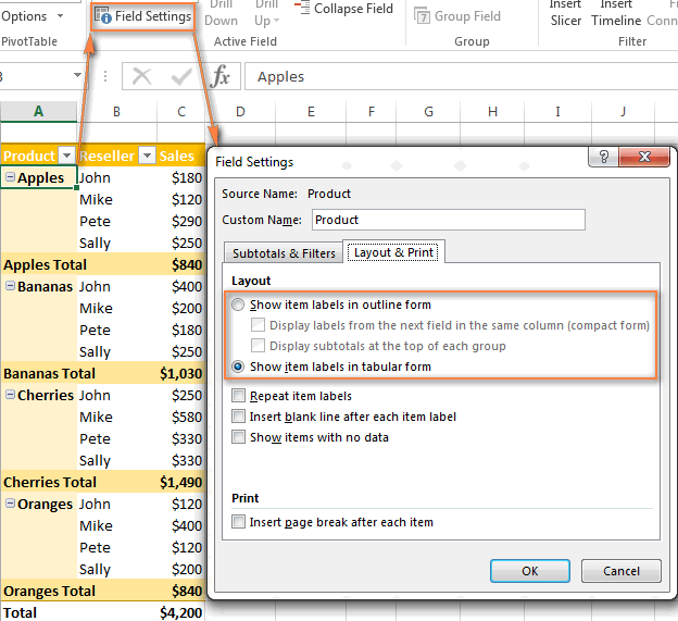
Excel Pivot Table tutorial – how to make and use PivotTables in Excel
How to change interval between labels in Excel 2013? I found the solution easily on the web. Just click on the axis on the chart -> then click on Format axis to the right -> Axis options -> Labels -> Under Interval between labels I should be able to specify interval units. In my case. There is No Interval Between Labels, it is missing. The only thing there is Label Position.

How to Create a Chart in Microsoft Excel - Tech Support
Format Data Label Options in PowerPoint 2013 for Windows Alternatively, select data labels of any data series in your chart and right-click to bring up a contextual menu, as shown in Figure 2, below. From this menu, choose the Format Data Labels option. Either of these options opens the Format Data Labels Task Pane, as shown in Figure 3, below.

Top 24 Weird Invention In Japan: How do change the default Excel spreadsheet download setting in ...
Format Data Labels in Excel- Instructions - TeachUcomp, Inc. To do this, click the "Format" tab within the "Chart Tools" contextual tab in the Ribbon. Then select the data labels to format from the "Chart Elements" drop-down in the "Current Selection" button group. Then click the "Format Selection" button that appears below the drop-down menu in the same area.
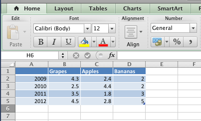
:max_bytes(150000):strip_icc()/EnterdatainExcel2003-5a5aa2b6d92b09003686c842.jpg)
How to Print Labels from Excel
Create Dynamic Chart Data Labels with Slicers - Excel Campus Feb 10, 2016 · Typically a chart will display data labels based on the underlying source data for the chart. In Excel 2013 a new feature called “Value from Cells” was introduced. This feature allows us to specify the a range that we want to use for the labels. Since our data labels will change between a currency ($) and percentage (%) formats, we need a ...
Legends in Excel Charts - Formats, Size, Shape, and Position - Peltier Tech Blog
Change the format of data labels in a chart To get there, after adding your data labels, select the data label to format, and then click Chart Elements > Data Labels > More Options. To go to the appropriate area, click one of the four icons ( Fill & Line , Effects , Size & Properties ( Layout & Properties in Outlook or Word), or Label Options ) shown here.

microsoft excel - Adding data label only to the last value - Super User
How to I rotate data labels on a column chart so that they are ... To change the text direction, first of all, please double click on the data label and make sure the data are selected (with a box surrounded like following image). Then on your right panel, the Format Data Labels panel should be opened. Go to Text Options > Text Box > Text direction > Rotate. And the text direction in the labels should be in ...
How To Add Data Labels To A Chart in Microsoft Excel - YouTube
Change the format of data labels in a chart To get there, after adding your data labels, select the data label to format, and then click Chart Elements > Data Labels > More Options. To go to the appropriate area, click one of the four icons ( Fill & Line, Effects, Size & Properties ( Layout & Properties in Outlook or Word), or Label Options) shown here.
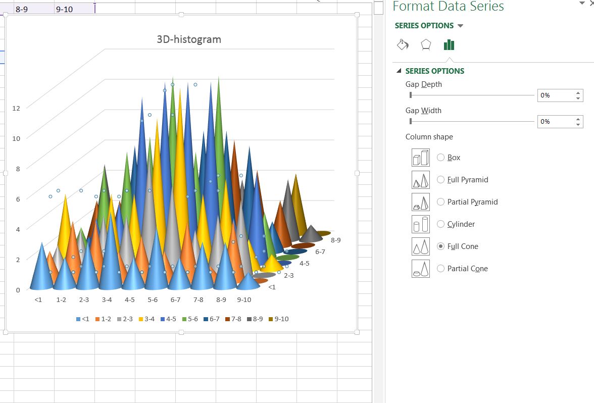
Advanced Graphs Using Excel : 3D-histogram in Excel
How to Change Excel Chart Data Labels to Custom Values? May 05, 2010 · Now, click on any data label. This will select “all” data labels. Now click once again. At this point excel will select only one data label. Go to Formula bar, press = and point to the cell where the data label for that chart data point is defined. Repeat the process for all other data labels, one after another. See the screencast.

excel - How do I update the data label of a chart? - Stack Overflow
How to change chart axis labels' font color and size in Excel? Right click the axis you will change labels when they are greater or less than a given value, and select the Format Axis from right-clicking menu. 2. Do one of below processes based on your Microsoft Excel version:

10 Ways Excel Pivot Tables Can Increase Your Productivity - BRAD EDGAR
Adding Colored Regions to Excel Charts - Duke Libraries Center for Data ... Nov 12, 2012 · Select any of the data series in the “Series” list, then go over to the “Category (X) axis labels” box and select the “Year” column. Click “OK”. Right-click on the x axis and select “Format Axis…”. Under “Scale”: Change the default interval between labels from 3 to 4; Change the interval between tick marks to 4 as well

How to Add Data Labels in Excel - Excelchat | Excelchat
Edit titles or data labels in a chart - support.microsoft.com Change the position of data labels. You can change the position of a single data label by dragging it. You can also place data labels in a standard position relative to their data markers. Depending on the chart type, you can choose from a variety of positioning options. On a chart, do one of the following:

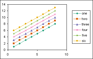
Excel chart type: How to create a variety of chart types
Edit titles or data labels in a chart - support.microsoft.com The first click selects the data labels for the whole data series, and the second click selects the individual data label. Right-click the data label, and then click Format Data Label or Format Data Labels. Click Label Options if it's not selected, and then select the Reset Label Text check box. Top of Page
Format Number Options for Chart Data Labels in Excel 2011 for Mac
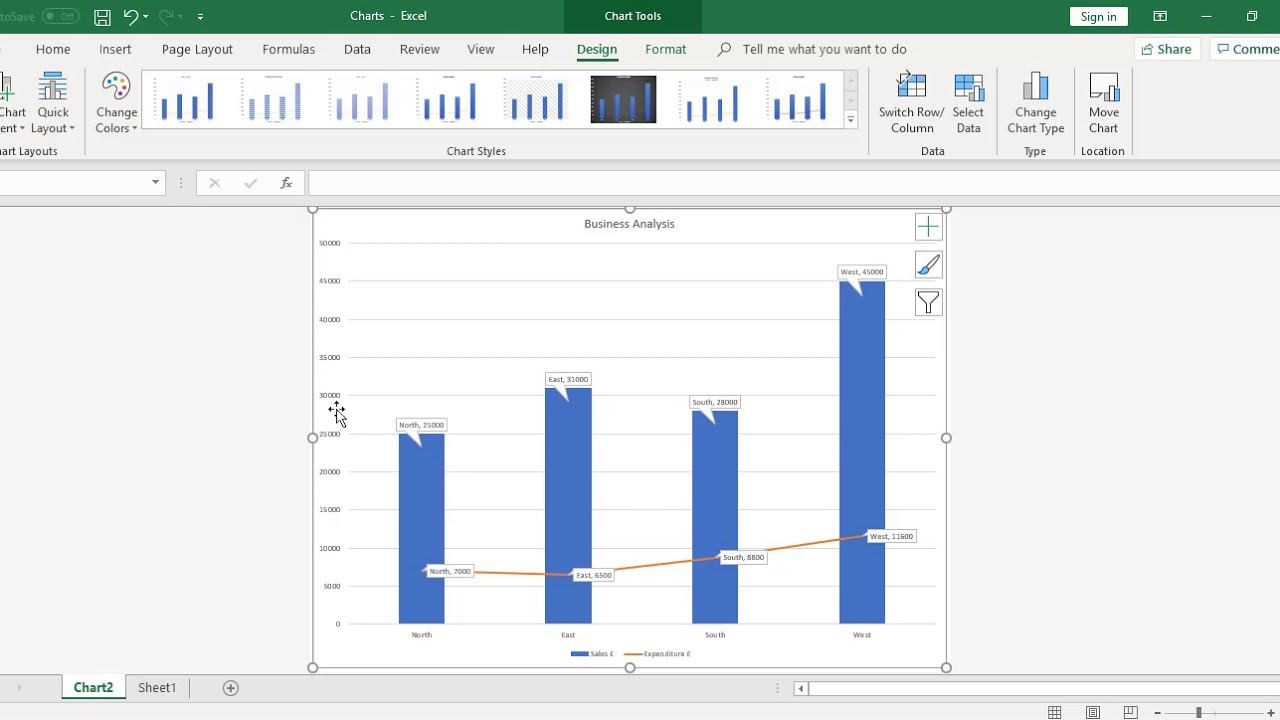
Add a Data Callout Label to Charts in Excel 2013 Dec 09, 2013 · The new Data Callout Labels make it easier to show the details about the data series or its individual data points in a clear and easy to read format. How to Add a Data Callout Label. Click on the data series or chart. In the upper right corner, next to your chart, click the Chart Elements button (plus sign), and then click Data Labels.

Show Trend Arrows in Excel Chart Data Labels | Excel, Chart, Excel tutorials
How to add data labels from different column in an Excel chart? Right click the data series, and select Format Data Labels from the context menu. 3. In the Format Data Labels pane, under Label Options tab, check the Value From Cells option, select the specified column in the popping out dialog, and click the OK button. Now the cell values are added before original data labels in bulk. 4.
Fixing Your Excel Chart When the Multi-Level Category Label Option is Missing. - Excel Dashboard ...
Add a Data Callout Label to Charts in Excel 2013 In the upper right corner, next to your chart, click the Chart Elements button (plus sign), and then click Data Labels. A right pointing arrow will appear, click on this arrow to view the submenu. Select Data Callout. Once the Data Callout Labels have been added, you can re-position them by clicking on their borders and dragging to a new position.

How to Add Data Labels to your Excel Chart in Excel 2013 - YouTube
How to Customize Your Excel Pivot Chart Data Labels - dummies To add data labels, just select the command that corresponds to the location you want. To remove the labels, select the None command. If you want to specify what Excel should use for the data label, choose the More Data Labels Options command from the Data Labels menu. Excel displays the Format Data Labels pane.
Post a Comment for "44 how to change data labels in excel 2013"