42 conditional formatting pivot table row labels

Conditional Formatting in a Pivot Table | MrExcel Message Board Those 3 scoping options are the ones described in the Microsoft link I referenced. Add, change, find, or clear conditional formats - Excel - Office.com. The step of: Home>Styles>Conditional Formatting>Manage Rules. Once here, there is a drop down at the top of the dialog box: "Show formatting rules for :". trumpexcel.com › replace-blank-cells-with-zerosHow to Replace Blank Cells with Zeros in Excel Pivot Tables Excel Pivot Tables has an option to quickly replace blank cells with zeroes. Here is how to do this: Right-click any cell in the Pivot Table and select Pivot Table Options. In Pivot Table Options Dialogue Box, within the Layout & Format tab, make sure that the For Empty cells show option is checked, and enter 0 in the field next to it.

Pivot Table Conditional Formatting for Different Rows Items? Hello, It is possible! All you have to do: Select Your Pivot Table and: Go to Conditional Formatting -> New Rule -> Choose All cells showing "duration" values for "Type and "Date Selection" under "Apply Rule To" section -> Use a Formula to Determine which cells to format and enter the following formula: =AND(A6="Cars",A6>3), You can create new rules for other two conditions as well:

Conditional formatting pivot table row labels

Apply Conditional Formatting | Excel Pivot Table Tutorial Go to Home Tab → Styles → Conditional Formatting → New Rule. From rule to, select the third option. And, from "select a rule" type select "Format only top or bottom" ranked values. In edit rule description, enter 1 in the input box and from the drop-down menu select "each Column Group". Apply formatting you want. Click OK. How to Replace Blank Cells with Zeros in Excel Pivot Tables In Pivot Table Options Dialogue Box, within the Layout & Format tab, make sure that the For Empty cells show option is checked, and enter 0 in the field next to it. If you want to can replace blank cells with text such as NA or No Sales. Click OK. That’s it! Now all the blank cells would automatically show 0. You can also play around with the ... Conditional formatting rows in a pivot table based on one rows criteria ... I am havong difficulty trying to highlight an entire row in a pivot table based on one rows criteria. The pivot table is from A:M and I need to highlight the corresponding row if column I has 992 in it. I have tried sevral ways but can only get it to work if I just focus on one row. I am at a loss for what I am doing wrong.

Conditional formatting pivot table row labels. peltiertech.com › pivot-chart-formatting-changesPivot Chart Formatting Changes When Filtered - Peltier Tech Apr 07, 2014 · Here is Jon A’s original unfiltered pivot table on the left and mine (Jon P’s) on the right. His has six columns of values, mine has two. There are several pivot charts below each pivot table. The first chart under each pivot table has only default formatting applied: blue for series 1, orange for series two, gray for series three, etc. Excel VBA: Conditional Format of Pivot Table based on Column Label ... myPivotSourceName = myPivotField.Name. Then rather than referencing the data field with the pivot field object, I referenced the DataRange with the string: myPivotTable.PivotFields (myPivotSourceName).DataRange.Select. Works perfectly and is completely portable for any pivottable on any sheet with any fields. excel vba. How to remove bold font of pivot table in Excel? - ExtendOffice The normal Bold feature can’t help us to un-bold the row labels in pivot table, but we can apply the powerful function – Conditional Formatting to solve this problem. Please do as follows: 1. Select the bold font row you want to un-bold in the pivot table, or you can press Ctrl key to select multiple bold font rows as your need. See screenshot: Pivot Table: Pivot table conditional formatting | Exceljet Select any cell in the data you wish to format and then choose "New rule" from the conditional formatting menu on the Home tab of the ribbon. At the top of the window, you will see setting for which cells to apply conditional formatting to. For the example shown, we want: "All cells showing sum of "sales values" for name and "date"

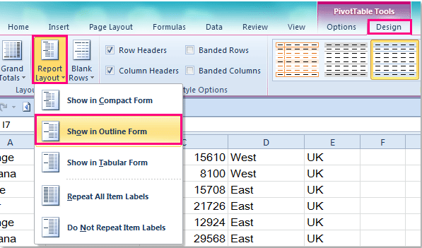
How to make row labels on same line in pivot table? - ExtendOffice Make row labels on same line with PivotTable Options You can also go to the PivotTable Options dialog box to set an option to finish this operation. 1. Click any one cell in the pivot table, and right click to choose PivotTable Options, see screenshot: 2. Design the layout and format of a PivotTable To change the format of the PivotTable, you can apply a predefined style, banded rows, and conditional formatting. Windows Web Mac Changing the layout form of a PivotTable Change a PivotTable to compact, outline, or tabular form Change the way item labels are displayed in a layout form Change the field arrangement in a PivotTable Add Pivot Table Conditional Formatting and Fix Problems To apply simple conditional formatting: In the pivot table, select the territory sales amounts, in cells B5:C16. On the Ribbon's Home tab, click Conditional Formatting. Click Top/Bottom Rules, and click Above Average. In the Above Average window, select one of the formatting options from the drop down list. Pivot Table Conditional Formatting Based on Another Column ... - ExcelDemy We can conditionally format the entire Pivot Table depending on the blanks. Step 1: Repeat Step 1 of Method 1 then the New Formatting Rule window will open. Here in the New Formatting Rule window, Select the 3rd and 2nd options from Apply Rule to and Select a Rule Type command box respectively. Inside Edit the Rule Description dialog box,

Formatting tables and pivot tables in Amazon QuickSight To add a label for totals and subtotals. In the Format visual pane, choose Total or Subtotal. For Label, enter a word or short phrase. In pivot tables, you can also add labels to column totals and subtotals. To do so, enter a word or short phrase for Label in the Columns section. To format totals and subtotals text. Format Pivot Table Labels Based on Date Range In the pivot table, remove any filters that have been applied - all the rows need to be visible before you apply the conditional formatting. Select all the dates in the Row Labels that you want to format. On the Ribbon, click the Home tab, and then in the Styles group, click Conditional Formatting. Conditional Format Pivot Table Row - Chandoo.org Select the entire row, and when you apply the conditional format, make the column reference absolute. So, say we want the entire row 2 to be formatted if cell in col B = 5. formula would be: =$B2=5 How to Apply Conditional Formatting to Pivot Tables 13.12.2018 · Great question! I don’t believe there is a direct way to do this with the conditional formatting setting for the pivot table. Those settings are applied at the pivot field level, and not the pivot item level. In the example of Quarters, each quarter (Q1, Q2, Q3, Q4) would be a pivot item. The conditional formatting is applied at the field level.

Finding Duplicates by Using Conditional Formatting in Excel 2010

Pivot Table Grouping, Ungrouping And Conditional Formatting #1) Select the entire column under the Sum of Total column in the pivot table. #2) Navigate to Home -> Conditional Formatting #3) Select Top/Bottom Rules -> Bottom 10 items. #4) In the dialog reduce the count to 3 (since we want just the bottom 3) and you can choose any highlighter from the drop-down.

Pivoting-tour

› pivot-tables › pivot-tableHow to Apply Conditional Formatting to Pivot Tables Dec 13, 2018 · Great question! I don’t believe there is a direct way to do this with the conditional formatting setting for the pivot table. Those settings are applied at the pivot field level, and not the pivot item level. In the example of Quarters, each quarter (Q1, Q2, Q3, Q4) would be a pivot item. The conditional formatting is applied at the field level.

Pin by Larry Xu on Excel | Pivot table, Excel, Row labels

How to apply conditional formatting to Pivot Tables - SpreadsheetWeb Go to HOME > Conditional Formatting > New Rule to add a new formatting rule, or select from predefined options. If you select the latter, you will need to configure the rule regardless. The New (or Edit) Formatting Rule window contains options specific to Pivot Tables. You can choose the location where you want to apply your conditional ...

dynamic - Conditional Formatting Pivot table in Google Sheets - Stack Overflow

Conditional formatting for Pivot Tables in Excel 2016 - 2007 - Ablebits Conditional formatting when applied to PivotTables in Excel 2007 - 2016 is applied to the underlying structure of the PivotTable rather than to the cells themselves. So, when you interact with a PivotTable such as moving fields around and viewing your data in different ways, the formatting is updated as you work.

Sorting a Pivot Table | MyExcelOnline

Conditional Formatting on Pivot Table row labels Re: Conditional Formatting on Pivot Table row labels Hi Dilip, The date is a "date" and not a text. What I mean is each cell in A should be compared with the 3 dates in E and should do the conditional formatting (excel icon sets) accordingly. If you see the cell A in srcFromWorkSheet you know what I mean. Please let me know if you have any queries.

85 DOWNLOAD PRINTABLE HOW DO I PIVOT TABLE IN EXCEL PDF DOC ZIP - Pivot

Re-Apply Pivot Table Conditional Formatting - yoursumbuddy In cases where the conditional formatting might not apply to the leftmost row label, I've still applied it to that column, but modified the condition to check which column it's in. This function can be modified and called from a SheetPivotTableUpdate event, so when users or code updates a pivot table it re-applies automatically.

pivot table - Conditional formatting between 2 sheets - Super User

› pivottabletextvaluesPivot Table Text Values - Contextures Excel Tips Jan 27, 2022 · On the Excel Ribbon's Home tab, click Conditional Formatting; Then click New Rule, to open the New Formatting Rule dialog box; In the Apply Rule to section, select the 3rd option - All cells showing 'Max of RegID' values for 'City' and 'Store'. This option creates flexible conditional formatting that will adjust if the pivot table layout changes.

How to repeat row labels for group in pivot table?

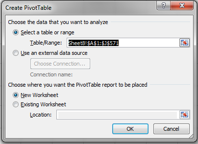
Conditional Formatting in Pivot Table - WallStreetMojo We must follow the steps to apply conditional formatting in the pivot table. First, we must select the data. Then, in the "Insert" Tab, click on "Pivot Tables." As a result, a dialog box appears. Next, we must insert the pivot table in a new worksheet by clicking "OK." Currently, a pivot table is blank. Next, we need to bring in the values.

Create Beautiful Reports with Custom Pivot Tables and JavaScript Spreadsheets | SpreadJS

Pivot Table Conditional Formatting with VBA - Peltier Tech Without resorting to macros, it's possible to quickly reapply the conditional format in 2007 by following these steps: - Set the conditional format to range covering more than the pivot table (e.g. on cell above). - When the pivot is refreshed, go to the "Conditional formatting Manage Rules…" dialog and edit the "Applies to" range.

How to Apply Conditional Formatting in Pivot Table? (with Example)

101 Advanced Pivot Table Tips And Tricks You Need To Know 25.04.2022 · Without a table your range reference will look something like above. In this example, if we were to add data past Row 51 or Column I our pivot table would not include it in the results. To create and name your table. Select your data. Go to the Insert tab and press the Table button in the Tables section, or use the keyboard shortcut Ctrl + T.

How To Find And Remove Duplicates In A Pivot Table - MS Excel | Excel In Excel

How to Filter Data in Pivot Table with Examples - EDUCBA Introduction to Pivot Table Filter. A Pivot Table filter is something that we get when we create a pivot table by default. First, create a table using a Pivot Table; we can see the first field, which is either a Row or Column, will have one filter. Click on the drop-down arrow or press the ALT + Down navigation key to go into the filter list ...

Conditional Formatting of Row in Text Table based on Dimension

conditional formatting per row on pivot - Microsoft Tech Community conditional formatting per row on pivot. I would like to format each row of a pivot table separately (as in the picture shown below), but I cannot paste the formatting. I've got many rows, and they could change (just like the columns) Is there a way to automate this, or I have to select row by row and apply the formatting?

Learn How to Apply Conditional Formatting in a Pivot Table | Excelchat

› pivot-table-filterPivot Table Filter | How to Filter Data in Pivot Table with ... Introduction to Pivot Table Filter. A Pivot Table filter is something that we get when we create a pivot table by default. First, create a table using a Pivot Table; we can see the first field, which is either a Row or Column, will have one filter. Click on the drop-down arrow or press the ALT + Down navigation key to go into the filter list.

Share :