45 how to add data labels in excel graph
› how-to-add-totals-toHow to Add Totals to Stacked Charts for Readability - Excel ... Make sure the chart is selected and add Center Data Labels from the Layout menu in Chart Tools. Now there are labels for all the bars in the chart, but the big total bars are still in our way. Select only the total bars in the chart. Then, go to the Format menu from the Chart Tools group. Click the Shape Fill drop-down and select No Fill. How to Add, Edit and Rename Data Labels in Excel Charts In this tutorial, you will learn how to add, edit and rename data labels in Microsoft excel graphs.#DataLabels #DataLabel #ExcelChart #ExcelGraph
learn.microsoft.com › en-us › deployofficeUse the Readiness Toolkit to assess application compatibility ... Oct 27, 2022 · For more information, see Use labels to categorize and filter data in reports. San Francisco : Label3 : Value of custom label, if configured. For more information, see Use labels to categorize and filter data in reports. Finance : Label4 : Value of custom label, if configured. For more information, see Use labels to categorize and filter data ...

How to add data labels in excel graph
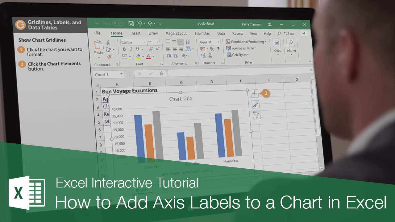
How to Add X and Y Axis Labels in Excel (2 Easy Methods) 2. Using Excel Chart Element Button to Add Axis Labels. In this second method, we will add the X and Y axis labels in Excel by Chart Element Button. In this case, we will label both the horizontal and vertical axis at the same time. The steps are: Steps: Firstly, select the graph. Secondly, click on the Chart Elements option and press Axis Titles. How to Add Two Data Labels In Excel Chart? - YouTube In this video tutorial, we are going to learn, how to add multiple data labels in excel pie chart.Our YouTube Channels Travel Volg Channelhttps:// ... How to Change the Data in Charts/Diagrams in PowerPoint Click on the chart. Go to Chart Design and click on Select Data. You will see a pop up box like the one shown above. In the Select Data Source pop up box follow the following instructions: To. Do This. Add a series. Under Legend Entries (Series), click the Add, and then add the data. Remove a series.
How to add data labels in excel graph. How to Add Two Data Labels in Excel Chart (with Easy Steps) Select the data labels. Then right-click your mouse to bring the menu. Format Data Labels side-bar will appear. You will see many options available there. Check Category Name. Your chart will look like this. Now you can see the category and value in data labels. Read More: How to Format Data Labels in Excel (with Easy Steps) Things to Remember How to Add Total Data Labels to the Excel Stacked Bar Chart Step 4: Right click your new line chart and select "Add Data Labels" Step 5: Right click your new data labels and format them so that their label position is "Above"; also make the labels bold and increase the font size. Step 6: Right click the line, select "Format Data Series"; in the Line Color menu, select "No line" Step 7 ... How To Add Data Labels In Excel - luanhong.us To do this, click the format tab within the chart tools contextual tab in the ribbon. Use the following steps to add data labels to series in a chart: Source: pakaccountants.com. Add custom data labels from the column x axis labels. In this second method, we will add the x and y axis labels in excel by chart element button. Add or remove data labels in a chart - support.microsoft.com Add data labels to a chart Click the data series or chart. To label one data point, after clicking the series, click that data point. In the upper right corner, next to the chart, click Add Chart Element > Data Labels. To change the location, click the arrow, and choose an option.
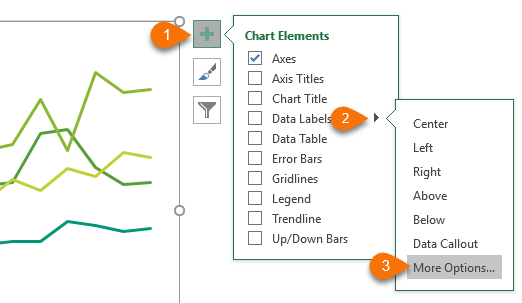
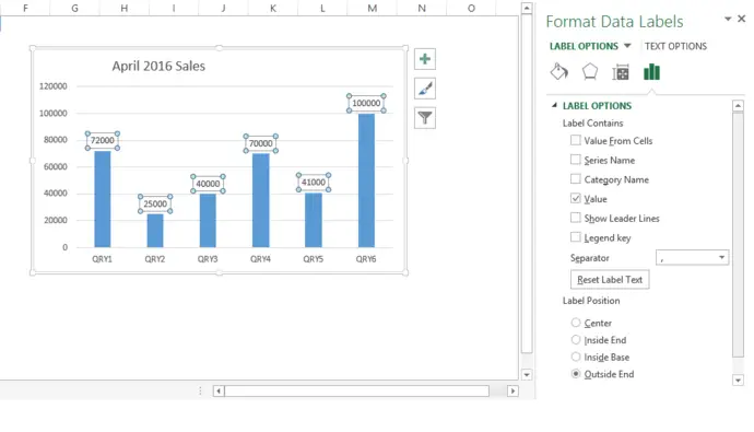
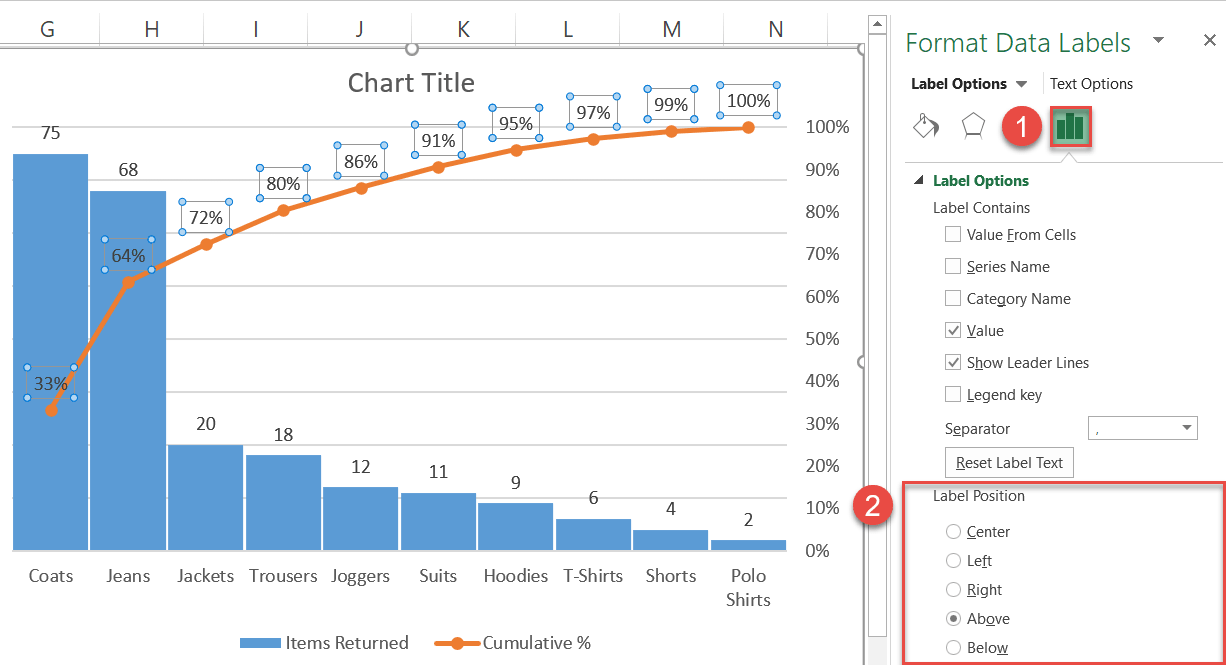
Data Labels in Excel Pivot Chart (Detailed Analysis) Next open Format Data Labels by pressing the More options in the Data Labels. Then on the side panel, click on the Value From Cells. Next, in the dialog box, Select D5:D11, and click OK. Right after clicking OK, you will notice that there are percentage signs showing on top of the columns. 4. Changing Appearance of Pivot Chart Labels › publication › 344638517_Excel(PDF) Excel For Statistical Data Analysis - ResearchGate Oct 14, 2020 · Start Excel, then click T ools and look for Data Analysis and for Solver. If both are there, press Esc (escape) If both are there, press Esc (escape) and continue with the respective assignment. Change the format of data labels in a chart To get there, after adding your data labels, select the data label to format, and then click Chart Elements > Data Labels > More Options. To go to the appropriate area, click one of the four icons ( Fill & Line, Effects, Size & Properties ( Layout & Properties in Outlook or Word), or Label Options) shown here. Excel Charts: Creating Custom Data Labels - YouTube In this video I'll show you how to add data labels to a chart in Excel and then change the range that the data labels are linked to. This video covers both W...
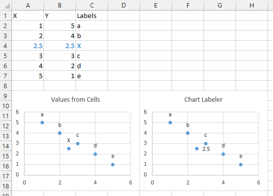
› how-to-select-best-excelBest Types of Charts in Excel for Data Analysis, Presentation ... Apr 29, 2022 · Use the moving average trendline if there is a lot of fluctuation in your data. How to add a chart to an Excel spreadsheet? To add a chart to an Excel spreadsheet, follow the steps below: Step-1: Open MS Excel and navigate to the spreadsheet, which contains the data table you want to use for creating a chart. Step-2: Select data for the chart: Edit titles or data labels in a chart - support.microsoft.com On a chart, click one time or two times on the data label that you want to link to a corresponding worksheet cell. The first click selects the data labels for the whole data series, and the second click selects the individual data label. Right-click the data label, and then click Format Data Label or Format Data Labels. Custom Chart Data Labels In Excel With Formulas - How To Excel At Excel Follow the steps below to create the custom data labels. Select the chart label you want to change. In the formula-bar hit = (equals), select the cell reference containing your chart label's data. In this case, the first label is in cell E2. Finally, repeat for all your chart laebls. How to Add Labels to Scatterplot Points in Excel - Statology Step 3: Add Labels to Points Next, click anywhere on the chart until a green plus (+) sign appears in the top right corner. Then click Data Labels, then click More Options… In the Format Data Labels window that appears on the right of the screen, uncheck the box next to Y Value and check the box next to Value From Cells.
Enable or Disable Excel Data Labels at the click of a button ...
Add a DATA LABEL to ONE POINT on a chart in Excel Click on the chart line to add the data point to. All the data points will be highlighted. Click again on the single point that you want to add a data label to. Right-click and select ' Add data label ' This is the key step! Right-click again on the data point itself (not the label) and select ' Format data label '.

How to Add Data Labels in Excel - Excelchat | Excelchat
Add or remove data labels in a chart - support.microsoft.com Depending on what you want to highlight on a chart, you can add labels to one series, all the series (the whole chart), or one data point. Add data labels. You can add data labels to show the data point values from the Excel sheet in the chart. This step applies to Word for Mac only: On the View menu, click Print Layout.

how to add data labels into Excel graphs — storytelling with data
support.microsoft.com › en-us › officeAdd or remove data labels in a chart - support.microsoft.com Depending on what you want to highlight on a chart, you can add labels to one series, all the series (the whole chart), or one data point. Add data labels. You can add data labels to show the data point values from the Excel sheet in the chart. This step applies to Word for Mac only: On the View menu, click Print Layout.

How to Add Total Data Labels to the Excel Stacked Bar Chart ...
How to Change the Data in Charts/Diagrams in PowerPoint Click on the chart. Go to Chart Design and click on Select Data. You will see a pop up box like the one shown above. In the Select Data Source pop up box follow the following instructions: To. Do This. Add a series. Under Legend Entries (Series), click the Add, and then add the data. Remove a series.

microsoft excel - Adding data label only to the last value ...
How to Add Two Data Labels In Excel Chart? - YouTube In this video tutorial, we are going to learn, how to add multiple data labels in excel pie chart.Our YouTube Channels Travel Volg Channelhttps:// ...

How to Add Two Data Labels in Excel Chart (with Easy Steps ...
How to Add X and Y Axis Labels in Excel (2 Easy Methods) 2. Using Excel Chart Element Button to Add Axis Labels. In this second method, we will add the X and Y axis labels in Excel by Chart Element Button. In this case, we will label both the horizontal and vertical axis at the same time. The steps are: Steps: Firstly, select the graph. Secondly, click on the Chart Elements option and press Axis Titles.

Excel charts: add title, customize chart axis, legend and ...
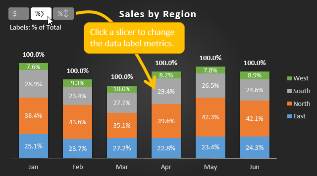
Create Dynamic Chart Data Labels with Slicers - Excel Campus

Adding rich data labels to charts in Excel 2013 | Microsoft ...

424 How to add data label to line chart in Excel 2016

How to Use Cell Values for Excel Chart Labels

Excel: Clustered Column Chart with Percent of Month ...

Chart Data Labels in PowerPoint 2011 for Mac

Apply Custom Data Labels to Charted Points - Peltier Tech
Dynamically Label Excel Chart Series Lines • My Online ...

How to Add and Remove Chart Elements in Excel

Custom Data Labels with Colors and Symbols in Excel Charts ...

Adding rich data labels to charts in Excel 2013 | Microsoft ...

How to Add Data Labels in Excel - Excelchat | Excelchat

Add Labels ON Your Bars

Add or remove data labels in a chart

How to Use Cell Values for Excel Chart Labels

Add or remove data labels in a chart

How to add live total labels to graphs and charts in Excel ...

Dynamically Label Excel Chart Series Lines • My Online ...
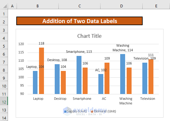
How to Add Two Data Labels in Excel Chart (with Easy Steps ...
Custom Chart Data Labels In Excel With Formulas
How to Add Axis Labels to a Chart in Excel | CustomGuide

how to add data labels into Excel graphs — storytelling with data

Custom data labels in a chart
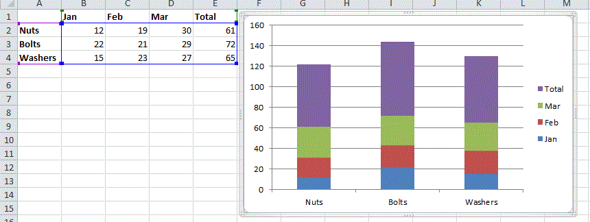
Excel Data Labels: How to add totals as labels to a stacked ...
Apply Custom Data Labels to Charted Points - Peltier Tech

Change the format of data labels in a chart

Creating Pie Chart and Adding/Formatting Data Labels (Excel)

How to Change Excel Chart Data Labels to Custom Values?

How to Customize Your Excel Pivot Chart Data Labels - dummies

Adding rich data labels to charts in Excel 2013 | Microsoft ...
How to Create a Pareto Chart in Excel – Automate Excel

Using the CONCAT function to create custom data labels for an ...

How-to Use Data Labels from a Range in an Excel Chart - Excel ...
How to Add Totals to Stacked Charts for Readability - Excel ...

Add Labels ON Your Bars

Add or remove data labels in a chart

data visualization - How do you put values over a simple bar ...

Directly Labeling Excel Charts - PolicyViz
Post a Comment for "45 how to add data labels in excel graph"